Alignment tutorial for two E15.5 Stereo-seq mouse embryo slices
In this tutorial, we will demonstrate how to implement two E15.5 mouse embryo slices alignment using 3d-OT and calculate the chamfer distance
Loading package
[1]:
from lib_3d_OT.utils import *
import scanpy as sc
import numpy as np
import pandas as pd
import torch
from lib_3d_OT.single_modialty import *
import torch.optim as optim
import warnings
warnings.filterwarnings("ignore")
During startup - Warning messages:
1: package ‘methods’ was built under R version 4.3.2
2: package ‘datasets’ was built under R version 4.3.2
3: package ‘utils’ was built under R version 4.3.2
4: package ‘grDevices’ was built under R version 4.3.2
5: package ‘graphics’ was built under R version 4.3.2
6: package ‘stats’ was built under R version 4.3.2
R[write to console]:                    __           __
   ____ ___  _____/ /_  _______/ /_
  / __ `__ \/ ___/ / / / / ___/ __/
 / / / / / / /__/ / /_/ (__  ) /_
/_/ /_/ /_/\___/_/\__,_/____/\__/   version 6.1.1
Type 'citation("mclust")' for citing this R package in publications.
[ ]:
device = torch.device("cuda:1" if torch.cuda.is_available() else "cpu")
Loading and Pre-processing two E15.5 Stereo-seq slices
First, we need to prepare the single cell spatial data into AnnData objects. AnnData is the standard data class we use in 3d-OT.
See documentation for more details if you are unfamiliar, including how to construct AnnData objects from scratch, and how to read data in other formats (csv, mtx, loom, etc.) into AnnData objects.
dpcais the preprocessing process for reference SLAT
[3]:
adata1=sc.read_h5ad('/home/dbj/mouse/oT/mouse/Chen-Stereo_seq-E15.5-s1.h5ad')
adata2=sc.read_h5ad('/home/dbj/mouse/oT/mouse/Chen-Stereo_seq-E15.5-s2.h5ad')
adata1.obs['truth']=adata1.obs['annotation']
adata2.obs['truth']=adata2.obs['annotation']
adatalist=[adata1,adata2]
adata1,adata2=dpca(adatalist,n_comps=50,join='inner')
Constructing neighbor graph and training the Pointnet++Encoder
We first build the neighbor graph graph1 of rep1 and train the encoder to get a trained encoder best_model1
[4]:
set_seed(7)
graph1 = prepare_data(adata2, location="spatial", nb_neighbors=8).to(device)
input_dim1 = graph1.express.shape[-1]
model1 = extractMODEL(args=None,input_dim=input_dim1)
optimizer = optim.Adam(model1.parameters(), lr=0.001)
best_model1, min_loss = train_graph_extractor(graph1, model1, optimizer, device,epochs=800)
Epoch 800/800, Loss: 1.076702, Min Loss: 1.072592
Constructing neighbor graph and training the Pointnet++Encoder
We then build the neighbor graph graph2 of rep2 and train the encoder to get a trained encoder best_model2
[5]:
set_seed(7)
graph2 = prepare_data(adata1, location="spatial", nb_neighbors=8).to(device)
input_dim2 = graph2.express.shape[-1]
model2 = extractMODEL(args=None, input_dim=input_dim2)
optimizer2 = optim.Adam(model2.parameters(), lr=0.001)
best_model2,min_loss = train_graph_extractor(graph2, model2,optimizer2, device, epochs=800)
Epoch 800/800, Loss: 1.057312, Min Loss: 1.049954
Training the optimal transport module
Enter graph1 and graph2 and the two encoders we trained into the optimal transport model
[6]:
pclouds_list=[graph1,graph2]
[24]:
set_seed(7)
input_dim1 = pclouds_list[0].express.shape[-1]
input_dim2 = pclouds_list[1].express.shape[-1]
model = UnifiedModel(input_dim1=input_dim1,input_dim2=input_dim2,simk=5,otk=300,reconk=1,best_encoder1=best_model1,best_encoder2=best_model2)
optimizer = torch.optim.Adam(model.parameters(), lr=0.0001)
lr_lambda = lambda epoch: 1.0 if epoch < 340 else 1.0
scheduler = torch.optim.lr_scheduler.LambdaLR(optimizer, lr_lambda)
args = {
    "backward_dist_weight":1.0,
    "use_smooth_flow":1,
    "smooth_flow_loss_weight":1.0,
    "use_div_flow":1,
    "div_flow_loss_weight":1.0,
    "div_neighbor": 8,
    "lattice_steps": 10,
    "nb_neigh_smooth_flow":32,
}


train(model=model,pcloud_list=pclouds_list,optimizer=optimizer,scheduler=scheduler,device=device,nb_epochs=1,use_corr_conf=False,use_smooth_flow=True,use_div_flow=True,args=args)
Time Pair 0,total_loss: 0.1472,smooth_flow_loss: 0.0912 Target Recon Loss: 0.00004472,Div Flow Loss: 0.0559
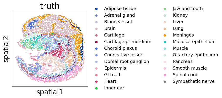
Source alignment slice
[8]:
import matplotlib.pyplot as plt
import copy
plt.rcParams['figure.figsize'] = (4,4)
plt.rcParams['font.size'] = 20
adata1_rotated = copy.deepcopy(adata1)
coords = adata1_rotated.obsm['spatial']

adata1_rotated.obsm['spatial'] = np.column_stack((coords[:, 0],-coords[:, 1]))
fig, ax = plt.subplots()
sc.pl.embedding(adata1_rotated,basis='spatial',color='truth',size=25,ax=ax,legend_fontsize=13)
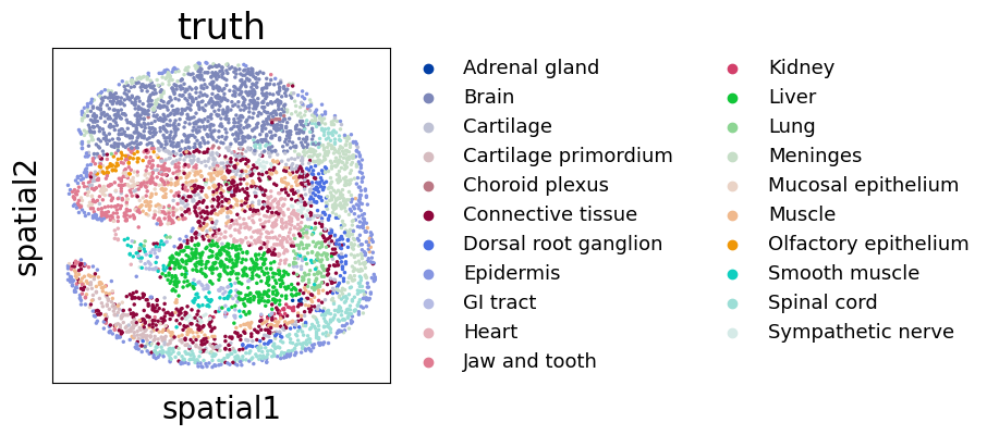
Target alignment slice
[9]:
import matplotlib.pyplot as plt
import copy
plt.rcParams['figure.figsize'] = (4,4)
plt.rcParams['font.size'] = 20
adata2_rotated = copy.deepcopy(adata2)
coords = adata2_rotated.obsm['spatial']

adata2_rotated.obsm['spatial'] = np.column_stack((coords[:, 0],-coords[:, 1]))
fig, ax = plt.subplots()
sc.pl.embedding(adata2_rotated,basis='spatial',color='truth',size=25,ax=ax,legend_fontsize=13)
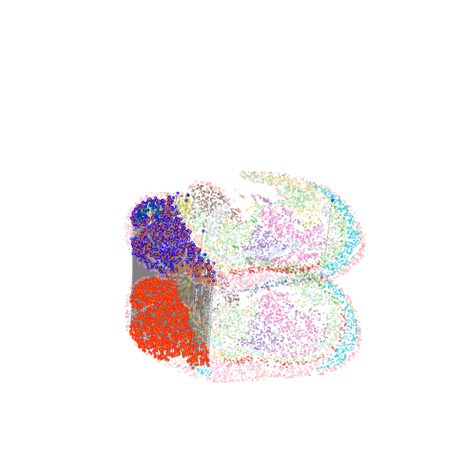
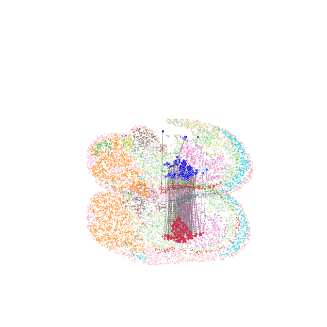
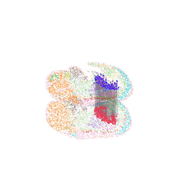
Visualize and quantify the evaluation of seven region alignment results
selected_cell_typerepresents the drawn source cell typefinaltruthmeans that the target cell type corresponding to the source cell type that based on the biological understanding, and it is used to obtain the spatial location information of the target cell type and calculate the chamfer distanceall_arrow_endsrepresents all aligned flow end positions from source cell type,it is used to calculate the chamfer distancelayer_1_pcloud_3Drepresents the target cell type spatial position information based on biological understanding, and is used to calculate the chamfer distance
[25]:
from lib_3d_OT.plot import *
all_arrow_ends,layer_1_pcloud_3D=plot_selected_cell_type_flow(pclouds_list, model, device,selected_cell_type='Brain',finaltruth=['Brain'],xlim=(-0.1, 1.1),ylim=(-0.1, 1.1),height_scale=1,size=1,alpha=0.4,
    #save_path='/home/dbj/DPLFC/'
)
Number of arrow ends: 1052
Layer 1 points count: 1063
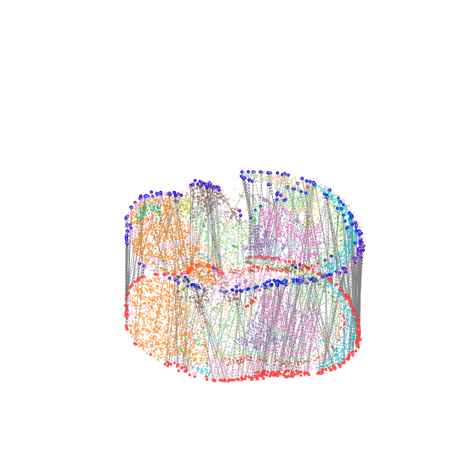
-Log10(chamfer_distance) as a performance metric for alignment
[26]:
chamfer_dist = chamfer_distance(all_arrow_ends,layer_1_pcloud_3D)

print(f"chamfer distance: {chamfer_dist}")
chamfer distance: 0.0005559758255398436
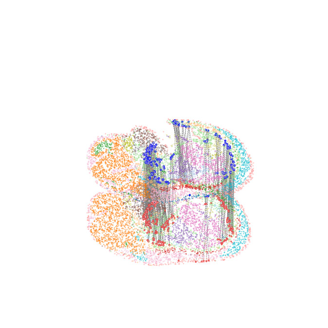
[27]:
from lib_3d_OT.plot import *
all_arrow_ends,layer_1_pcloud_3D=plot_selected_cell_type_flow(pclouds_list, model, device,selected_cell_type='Epidermis',finaltruth=['Epidermis'],xlim=(-0.1, 1.1),ylim=(-0.1, 1.1),height_scale=1,size=1,alpha=0.4,
    #save_path='/home/dbj/DPLFC/'
)
Number of arrow ends: 382
Layer 1 points count: 350
[28]:
chamfer_dist = chamfer_distance(all_arrow_ends,layer_1_pcloud_3D)

print(f"chamfer distance: {chamfer_dist}")
chamfer distance: 0.0035619710656050936
[29]:
from lib_3d_OT.plot import *
all_arrow_ends,layer_1_pcloud_3D=plot_selected_cell_type_flow(pclouds_list, model, device,selected_cell_type='Heart',finaltruth=['Heart'],xlim=(-0.1, 1.1),ylim=(-0.1, 1.1),height_scale=1,size=1,alpha=0.4,
    #save_path='/home/dbj/DPLFC/'
)
Number of arrow ends: 214
Layer 1 points count: 222
[30]:
chamfer_dist = chamfer_distance(all_arrow_ends,layer_1_pcloud_3D)

print(f"chamfer distance: {chamfer_dist}")
chamfer distance: 0.0037783370197349017
[31]:
from lib_3d_OT.plot import *
all_arrow_ends,layer_1_pcloud_3D=plot_selected_cell_type_flow(pclouds_list, model, device,selected_cell_type='Muscle',finaltruth=['Muscle'],xlim=(-0.1, 1.1),ylim=(-0.1, 1.1),height_scale=1,size=1,alpha=0.4,
    #save_path='/home/dbj/DPLFC/'
)
Number of arrow ends: 290
Layer 1 points count: 376
[32]:
chamfer_dist = chamfer_distance(all_arrow_ends,layer_1_pcloud_3D)

print(f"chamfer distance: {chamfer_dist}")
chamfer distance: 0.00018840872474427232
[33]:
from lib_3d_OT.plot import *
all_arrow_ends,layer_1_pcloud_3D=plot_selected_cell_type_flow(pclouds_list, model, device,selected_cell_type='Spinal cord',finaltruth=['Spinal cord'],xlim=(-0.1, 1.1),ylim=(-0.1, 1.1),height_scale=1,size=1,alpha=0.4,
    #save_path='/home/dbj/DPLFC/'
)
Number of arrow ends: 302
Layer 1 points count: 371
[34]:
chamfer_dist = chamfer_distance(all_arrow_ends,layer_1_pcloud_3D)

print(f"chamfer distance: {chamfer_dist}")
chamfer distance: 0.00034934705868540816
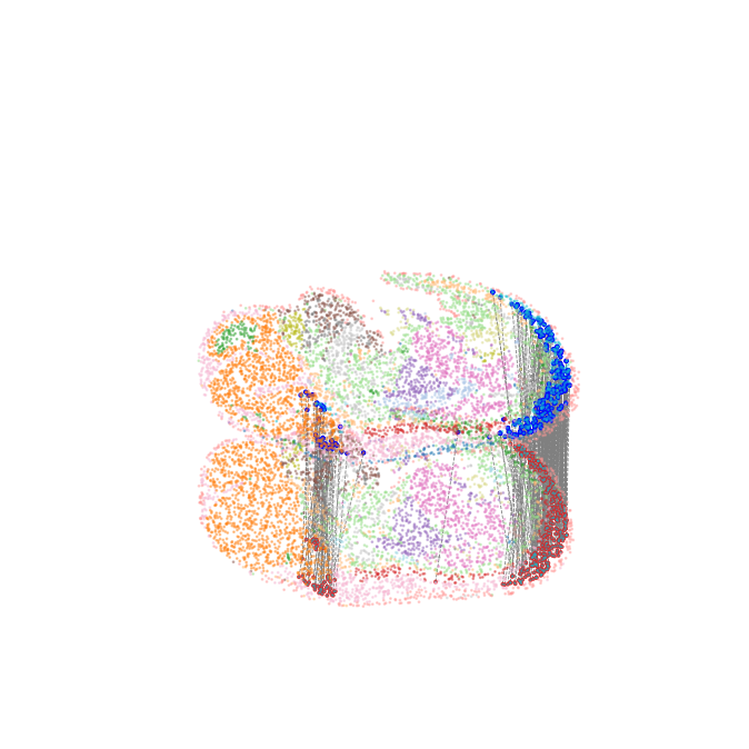
[35]:
from lib_3d_OT.plot import *
all_arrow_ends,layer_1_pcloud_3D=plot_selected_cell_type_flow(pclouds_list, model, device,selected_cell_type='Connective tissue',finaltruth=['Connective tissue'],xlim=(-0.1, 1.1),ylim=(-0.1, 1.1),height_scale=1,size=1,alpha=0.4,
    #save_path='/home/dbj/DPLFC/'
)
Number of arrow ends: 627
Layer 1 points count: 847
[36]:
chamfer_dist = chamfer_distance(all_arrow_ends,layer_1_pcloud_3D)

print(f"chamfer distance: {chamfer_dist}")
chamfer distance: 0.0008761489905992954
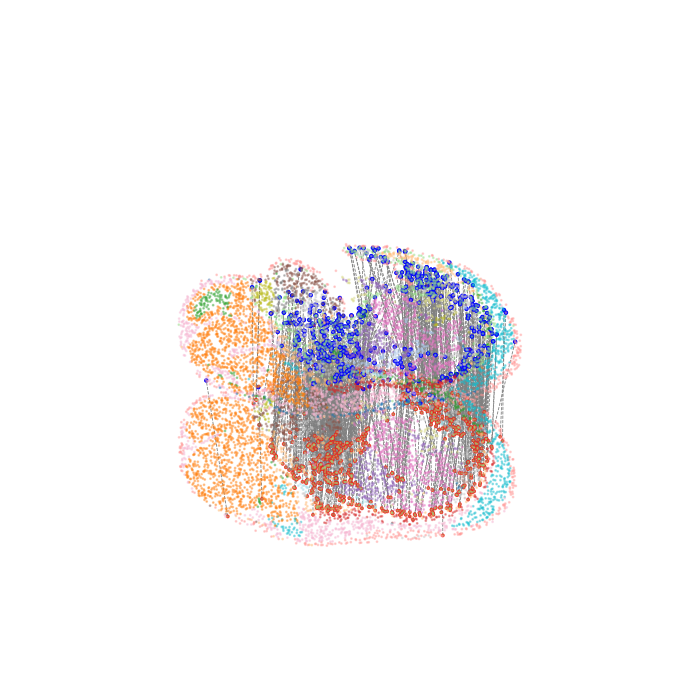
[37]:
from lib_3d_OT.plot import *
all_arrow_ends,layer_1_pcloud_3D=plot_selected_cell_type_flow(pclouds_list, model, device,selected_cell_type='Liver',finaltruth=['Liver'],xlim=(-0.1, 1.1),ylim=(-0.1, 1.1),height_scale=1,size=1,alpha=0.4,
    #save_path='/home/dbj/DPLFC/'
)
Number of arrow ends: 402
Layer 1 points count: 369
[38]:
chamfer_dist = chamfer_distance(all_arrow_ends,layer_1_pcloud_3D)

print(f"chamfer distance: {chamfer_dist}")
chamfer distance: 0.00015183553451676208