Alignment tutorial for 151673 and 151674 from DLPFC

In this tutorial, we will demonstrate how to implement 151673 and 151674 alignment using 3d-OT and calculate the chamfer distance

Loading package

from lib_3d_OT.utils import *
import scanpy as sc
import numpy as np
import pandas as pd
import torch
from lib_3d_OT.single_modialty import *
import torch.optim as optim
import warnings
warnings.filterwarnings("ignore")

During startup - Warning messages:
1: package ‘methods’ was built under R version 4.3.2
2: package ‘datasets’ was built under R version 4.3.2
3: package ‘utils’ was built under R version 4.3.2
4: package ‘grDevices’ was built under R version 4.3.2
5: package ‘graphics’ was built under R version 4.3.2
6: package ‘stats’ was built under R version 4.3.2
R[write to console]:                    __           __
   ____ ___  _____/ /_  _______/ /_
  / __ `__ \/ ___/ / / / / ___/ __/
 / / / / / / /__/ / /_/ (__  ) /_
/_/ /_/ /_/\___/_/\__,_/____/\__/   version 6.1.1
Type 'citation("mclust")' for citing this R package in publications.

device = torch.device("cuda:1" if torch.cuda.is_available() else "cpu")

Loading and Pre-processing two slices from 151673 and 151674

• First, we need to prepare the single cell spatial data into AnnData objects. AnnData is the standard data class we use in 3d-OT.

• See documentation for more details if you are unfamiliar, including how to construct AnnData objects from scratch, and how to read data in other formats (csv, mtx, loom, etc.) into AnnData objects.

• dpca is the preprocessing process for reference SLAT.

adata1=sc.read_visium('/home/dbj/mouse/DLPFC/DLPFC/151673/')
adata1.var_names_make_unique()
truth = pd.read_csv('/home/dbj/mouse/vision/spatial/DLPFC_annotations/151673_truth.csv', sep='\t', index_col=0)
adata1.obs['truth'] = truth.iloc[:,0]
adata1 = adata1[~adata1.obs['truth'].isna(), :]

adata2=sc.read_visium('/home/dbj/mouse/DLPFC/DLPFC/151674/')
adata2.var_names_make_unique()
truth = pd.read_csv('/home/dbj/mouse/vision/spatial/DLPFC_annotations/151674_truth.csv', sep='\t', index_col=0)
adata2.obs['truth'] = truth.iloc[:,0]
adata2 = adata2[~adata2.obs['truth'].isna(), :]

adatalist=[adata1,adata2]
adata1,adata2=dpca(adatalist,n_comps=50,join='inner')

Constructing neighbor graph and training the Pointnet++Encoder

We first build the neighbor graph graph1 of 151673 and train the encoder to get a trained encoder best_model1

set_seed(7)
graph1 = prepare_data(adata1, location="spatial", nb_neighbors=8).to(device)
input_dim1 = graph1.express.shape[-1]
model = extractMODEL(args=None,input_dim=input_dim1)
optimizer = optim.Adam(model.parameters(), lr=0.001)
best_model1, min_loss = train_graph_extractor(graph1, model, optimizer, device,epochs=800)

Epoch 800/800, Loss: 2.200454, Min Loss: 2.212034

Constructing neighbor graph and training the Pointnet++Encoder

We then build the neighbor graph graph2 of 151674 and train the encoder to get a trained encoder best_model2

set_seed(7)
graph2 = prepare_data(adata2, location="spatial", nb_neighbors=8).to(device)
input_dim2 = graph2.express.shape[-1]
model = extractMODEL(args=None,input_dim=input_dim2)
optimizer = optim.Adam(model.parameters(), lr=0.001)
best_model2, min_loss = train_graph_extractor(graph2, model, optimizer, device,epochs=800)

Epoch 800/800, Loss: 2.350463, Min Loss: 2.356186

Source align slice truth

import matplotlib.pyplot as plt
import copy
plt.rcParams['figure.figsize'] = (4,4)
plt.rcParams['font.size'] = 20
adata1_rotated = copy.deepcopy(adata1)
coords = adata1_rotated.obsm['spatial']

adata1_rotated.obsm['spatial'] = np.column_stack((coords[:, 0],-coords[:, 1]))
fig, ax = plt.subplots()
sc.pl.embedding(adata1_rotated,basis='spatial',color='truth',size=45,ax=ax)

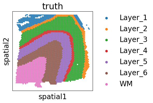
Target align slice truth

import matplotlib.pyplot as plt
import copy
plt.rcParams['figure.figsize'] = (4,4)
plt.rcParams['font.size'] = 20
adata2_rotated = copy.deepcopy(adata2)
coords = adata2_rotated.obsm['spatial']

adata2_rotated.obsm['spatial'] = np.column_stack((coords[:, 0],-coords[:, 1]))
fig, ax = plt.subplots()
sc.pl.embedding(adata2_rotated,basis='spatial',color='truth',size=45,ax=ax)

Training the optimal transport module

Enter graph1 and graph2 and the two encoders we trained into the optimal transport model

pclouds_list=[graph1,graph2]

input_dim1 = pclouds_list[0].express.shape[-1]
input_dim2 = pclouds_list[1].express.shape[-1]
model = UnifiedModel(input_dim1=input_dim1,input_dim2=input_dim2,simk=5,otk=20,reconk=1,best_encoder1=best_model1,best_encoder2=best_model2)
optimizer = torch.optim.Adam(model.parameters(), lr=0.0001)
lr_lambda = lambda epoch: 1.0 if epoch < 340 else 1.0
scheduler = torch.optim.lr_scheduler.LambdaLR(optimizer, lr_lambda)
args = {
    "backward_dist_weight":1.0,
    "use_smooth_flow":1,
    "smooth_flow_loss_weight":1.0,
    "use_div_flow":1,
    "div_flow_loss_weight":1.0,
    "div_neighbor": 8,
    "lattice_steps": 10,
    "nb_neigh_smooth_flow":32,
}



train(model=model,pcloud_list=pclouds_list,optimizer=optimizer,scheduler=scheduler,device=device,nb_epochs=1,use_corr_conf=False,use_smooth_flow=True,use_div_flow=True,args=args)

Time Pair 0,total_loss: 0.0586,smooth_flow_loss: 0.0404 Target Recon Loss: 0.00010402,Div Flow Loss: 0.0181

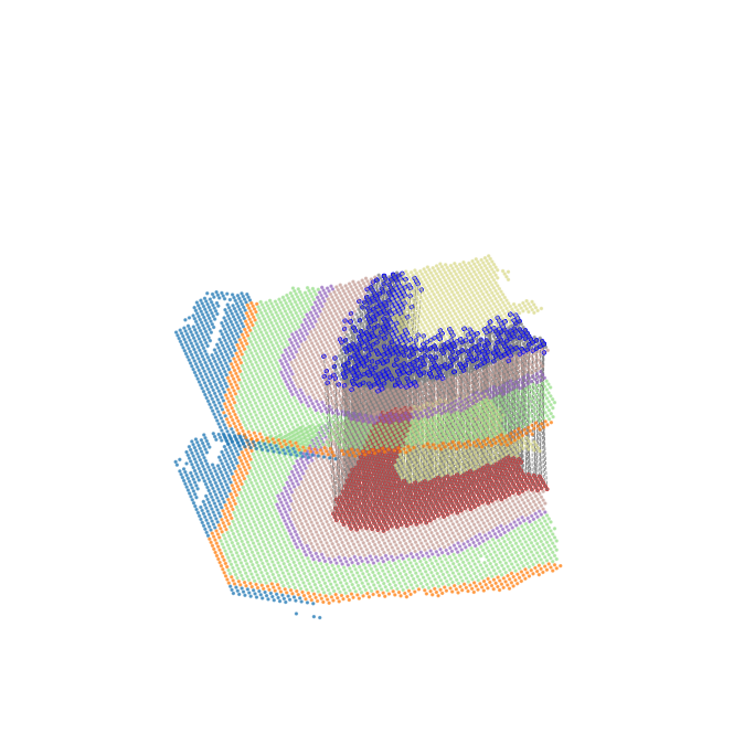
Visualize and quantify the evaluation of seven region alignment results

• selected_cell_type represents the drawn source cell type

• finaltruth means that the target cell type corresponding to the source cell type that based on the biological understanding, and it is used to obtain the spatial location information of the target cell type and calculate the chamfer distance

• all_arrow_ends represents all aligned flow end positions from source cell type,it is used to calculate the chamfer distance

• layer_1_pcloud_3D represents the target cell type spatial position information based on biological understanding, and is used to calculate the chamfer distance

Layer_1 alignment result

from lib_3d_OT.plot import *
all_arrow_ends,layer_1_pcloud_3D=plot_selected_cell_type_flow(pclouds_list, model, device,selected_cell_type='Layer_1',finaltruth=['Layer_1'],xlim=(-0.1, 1.1),ylim=(-0.1, 1.1),height_scale=1,size=2,alpha=0.6,
    #save_path='/home/dbj/DPLFC/'
)

Number of arrow ends: 273
Layer 1 points count: 380

-Log10(chamfer_distance) as a performance metric for alignment

chamfer_dist = chamfer_distance(all_arrow_ends,layer_1_pcloud_3D)

print(f"chamfer distance: {chamfer_dist}")

chamfer distance: 0.0003613015316660893

Layer_2 alignment result

from lib_3d_OT.plot import *
all_arrow_ends,layer_1_pcloud_3D=plot_selected_cell_type_flow(pclouds_list, model, device,selected_cell_type='Layer_2',finaltruth=['Layer_2'],xlim=(-0.1, 1.1),ylim=(-0.1, 1.1),height_scale=1,size=2,alpha=0.6,
    #save_path='/home/dbj/DPLFC/'
)

Number of arrow ends: 253
Layer 1 points count: 224

chamfer_dist = chamfer_distance(all_arrow_ends,layer_1_pcloud_3D)

print(f"chamfer distance: {chamfer_dist}")

chamfer distance: 0.0003549892395294974

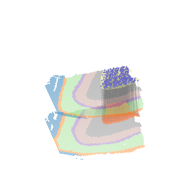
Layer_3 alignment result

from lib_3d_OT.plot import *
all_arrow_ends,layer_1_pcloud_3D=plot_selected_cell_type_flow(pclouds_list, model, device,selected_cell_type='Layer_3',finaltruth=['Layer_3'],xlim=(-0.1, 1.1),ylim=(-0.1, 1.1),height_scale=1,size=2,alpha=0.6,
    #save_path='/home/dbj/DPLFC/'
)

Number of arrow ends: 988
Layer 1 points count: 923

chamfer_dist = chamfer_distance(all_arrow_ends,layer_1_pcloud_3D)

print(f"chamfer distance: {chamfer_dist}")

chamfer distance: 0.0003613015316660893

Layer_4 alignment result

from lib_3d_OT.plot import *
all_arrow_ends,layer_1_pcloud_3D=plot_selected_cell_type_flow(pclouds_list, model, device,selected_cell_type='Layer_4',finaltruth=['Layer_4'],xlim=(-0.1, 1.1),ylim=(-0.1, 1.1),height_scale=1,size=2,alpha=0.6,
    #save_path='/home/dbj/DPLFC/'
)

Number of arrow ends: 218
Layer 1 points count: 247

chamfer_dist = chamfer_distance(all_arrow_ends,layer_1_pcloud_3D)

print(f"chamfer distance: {chamfer_dist}")

chamfer distance: 0.0004005055165088926

Layer_5 alignment result

from lib_3d_OT.plot import *
all_arrow_ends,layer_1_pcloud_3D=plot_selected_cell_type_flow(pclouds_list, model, device,selected_cell_type='Layer_5',finaltruth=['Layer_5'],xlim=(-0.1, 1.1),ylim=(-0.1, 1.1),height_scale=1,size=2,alpha=0.6,
    #save_path='/home/dbj/DPLFC/'
)

Number of arrow ends: 673
Layer 1 points count: 621

chamfer_dist = chamfer_distance(all_arrow_ends,layer_1_pcloud_3D)

print(f"chamfer distance: {chamfer_dist}")

chamfer distance: 0.0002188742874835671

Layer_6 alignment result

from lib_3d_OT.plot import *
all_arrow_ends,layer_1_pcloud_3D=plot_selected_cell_type_flow(pclouds_list, model, device,selected_cell_type='Layer_6',finaltruth=['Layer_6'],xlim=(-0.1, 1.1),ylim=(-0.1, 1.1),height_scale=1,size=2,alpha=0.6,
    #save_path='/home/dbj/DPLFC/'
)

Number of arrow ends: 692
Layer 1 points count: 614

chamfer_dist = chamfer_distance(all_arrow_ends,layer_1_pcloud_3D)

print(f"chamfer distance: {chamfer_dist}")

chamfer distance: 0.00039949498587779836

WM alignment result

from lib_3d_OT.plot import *
all_arrow_ends,layer_1_pcloud_3D=plot_selected_cell_type_flow(pclouds_list, model, device,selected_cell_type='WM',finaltruth=['WM'],xlim=(-0.1, 1.1),ylim=(-0.1, 1.1),height_scale=1,size=2,alpha=0.6,
    #save_path='/home/dbj/DPLFC/'
)

Number of arrow ends: 513
Layer 1 points count: 625

chamfer_dist = chamfer_distance(all_arrow_ends,layer_1_pcloud_3D)

print(f"chamfer distance: {chamfer_dist}")

chamfer distance: 0.00018394429114206693