Cross_platform

Alignment tutorial for seq-FISH and Stereo-seq

In this tutorial, we will demonstrate how to implement cross-platform alignment using 3d-OT and calculate the chamfer distance.

Loading package

from lib_3d_OT.utils import *
import scanpy as sc
import numpy as np
import pandas as pd
import torch
from lib_3d_OT.single_modialty import *
import torch.optim as optim
import warnings
warnings.filterwarnings("ignore")

During startup - Warning messages:
1: package ‘methods’ was built under R version 4.3.2
2: package ‘datasets’ was built under R version 4.3.2
3: package ‘utils’ was built under R version 4.3.2
4: package ‘grDevices’ was built under R version 4.3.2
5: package ‘graphics’ was built under R version 4.3.2
6: package ‘stats’ was built under R version 4.3.2
R[write to console]:                    __           __
   ____ ___  _____/ /_  _______/ /_
  / __ `__ \/ ___/ / / / / ___/ __/
 / / / / / / /__/ / /_/ (__  ) /_
/_/ /_/ /_/\___/_/\__,_/____/\__/   version 6.1.1
Type 'citation("mclust")' for citing this R package in publications.

Could not load compiled 3D CUDA chamfer distance

device = torch.device("cuda:1" if torch.cuda.is_available() else "cpu")

1. Loading and Pre-processing two slices from E8.75seq-FISH mouse embryo and E9.5 Stereo-seq mouse embryo

• First, we need to prepare the single cell spatial data into AnnData objects. AnnData is the standard data class we use in 3d-OT.

• See documentationfor more details if you are unfamiliar, including how to construct AnnData objects from scratch, and how to read data in other formats (csv, mtx, loom, etc.) into AnnData objects.

• dpca is the preprocessing process for reference SLAT.

adata1=sc.read_h5ad('/home/dbj/mouse/seq-flash/adata_seqFISH_mouse_E8.75.h5ad')
adata1.obs['truth']=adata1.obs['celltype']
adata2=sc.read_h5ad('/home/dbj/mouse/oT/different-time/E9.5.h5ad')
adata2.obs['truth']=adata2.obs['annotation']
adatalist=[adata1,adata2]
adata1,adata2=dpca(adatalist,n_comps=50,join='inner')

2. Constructing neighbor graph and training the Pointnet++Encoder

• We first build the mouse embryo graph structure graph1 of Stereo-seq E9.5 and train the encoder to get a trained encoder best_model1.

set_seed(7)
graph1 = prepare_data(adata2, location="spatial", nb_neighbors=8).to(device)
input_dim1 = graph1.express.shape[-1]
model1 = extractMODEL(args=None,input_dim=input_dim1)
optimizer = optim.Adam(model1.parameters(), lr=0.001)
best_model1, min_loss = train_graph_extractor(graph1, model1, optimizer, device,epochs=1150)

Epoch 1150/1150, Loss: 0.396464, Min Loss: 0.397595

• Building the mouse embryo graph structure graph2 of seq-FISH E8.75 and train the encoder to get a trained encoder best_model2.

set_seed(7)
graph2 = prepare_data(adata1, location="spatial", nb_neighbors=8).to(device)
input_dim2 = graph2.express.shape[-1]
model2 = extractMODEL(args=None, input_dim=input_dim2)
optimizer2 = optim.Adam(model2.parameters(), lr=0.001)
best_model2,min_loss = train_graph_extractor(graph2, model2,optimizer2, device, epochs=500)

Epoch 500/500, Loss: 0.422382, Min Loss: 0.422330

Training the optimal transport module

• Enter graph1 and graph2 and the two encoders we trained into the optimal transport model.

pclouds_list=[graph1,graph2]

input_dim1 = pclouds_list[0].express.shape[-1]
input_dim2 = pclouds_list[1].express.shape[-1]
model = UnifiedModel(input_dim1=input_dim1,input_dim2=input_dim2,simk=5,otk=2000,reconk=1,best_encoder1=best_model1,best_encoder2=best_model2)
optimizer = torch.optim.Adam(model.parameters(), lr=0.0001)
lr_lambda = lambda epoch: 1.0 if epoch < 340 else 1.0
scheduler = torch.optim.lr_scheduler.LambdaLR(optimizer, lr_lambda)
args = {
    "backward_dist_weight":1.0,
    "use_smooth_flow":1,
    "smooth_flow_loss_weight":1.0,
    "use_div_flow":1,
    "div_flow_loss_weight":1.0,
    "div_neighbor": 8,
    "lattice_steps": 10,
    "nb_neigh_smooth_flow":32,
}



train(model=model,pcloud_list=pclouds_list,optimizer=optimizer,scheduler=scheduler,device=device,use_corr_conf=False,use_smooth_flow=True,use_div_flow=True,args=args)

Time Pair 0,total_loss: 0.2421,smooth_flow_loss: 0.1522 Target Recon Loss: 0.00004927,Div Flow Loss: 0.0899

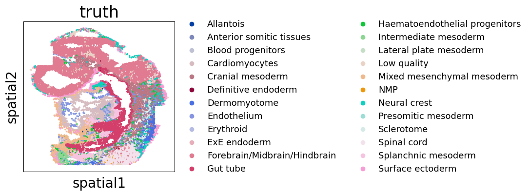
Target align slice truth

import matplotlib.pyplot as plt
import copy
plt.rcParams['figure.figsize'] = (4,4)
plt.rcParams['font.size'] = 20
adata1_rotated = copy.deepcopy(adata1)
coords = adata1_rotated.obsm['spatial']
adata1_rotated.obsm['spatial'] = np.column_stack((coords[:, 0],-coords[:, 1]))
fig, ax = plt.subplots()
sc.pl.embedding(adata1_rotated,basis='spatial',color='truth',size=25,ax=ax,legend_fontsize=13)

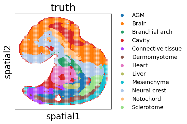
Source align slice truth

import matplotlib.pyplot as plt
import copy
plt.rcParams['figure.figsize'] = (4,4)
plt.rcParams['font.size'] = 20
adata2_rotated = copy.deepcopy(adata2)
coords = adata2_rotated.obsm['spatial']

adata2_rotated.obsm['spatial'] = np.column_stack((coords[:, 0],-coords[:, 1]))
fig, ax = plt.subplots()
sc.pl.embedding(adata2_rotated,basis='spatial',color='truth',size=25,ax=ax,legend_fontsize=13)

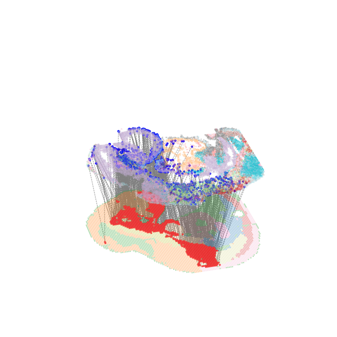
Visualize and quantify the evaluation of Brain region alignment results

• selected_cell_type represents the drawn source cell type.

• finaltruth means that the target cell type corresponding to the source cell type that based on the biological understanding, and it is used to obtain the spatial location information of the target cell type and calculate the chamfer distance.

• all_arrow_ends represents all aligned flow end positions from source cell type,it is used to calculate the chamfer distance.

• layer_1_pcloud_3D represents the target cell type spatial position information based on biological understanding, and is used to calculate the chamfer distance.

from lib_3d_OT.plot import *
all_arrow_ends,layer_1_pcloud_3D=plot_selected_cell_type_flow(pclouds_list, model, device,selected_cell_type='Brain',finaltruth=['Forebrain/Midbrain/Hindbrain'],xlim=(-0.1, 1.1),ylim=(-0.1, 1.1),height_scale=1,size=1,alpha=0.2,
    #save_path='/home/dbj/DPLFC/'
)

Number of arrow ends: 1518
Layer 1 points count: 4875

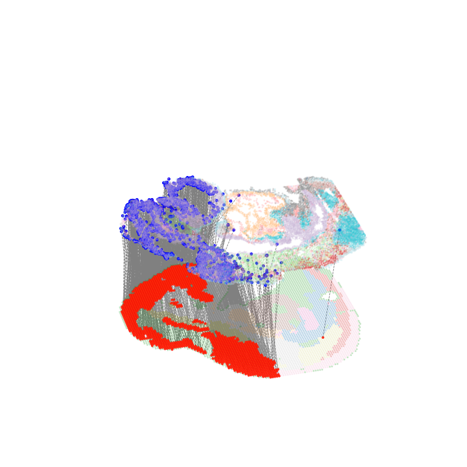
• -Log10(chamfer_distance) as a performance metric for alignment

chamfer_dist = chamfer_distance(all_arrow_ends,layer_1_pcloud_3D)

print(f"chamfer distance: {chamfer_dist}")

chamfer distance: 0.0005038145163827955

Visualize and quantify the evaluation of Heart region alignment results

from lib_3d_OT.plot import *
all_arrow_ends,layer_1_pcloud_3D=plot_selected_cell_type_flow(pclouds_list, model, device,selected_cell_type='Heart',finaltruth=['Cardiomyocytes'],xlim=(-0.1, 1.1),ylim=(-0.1, 1.1),height_scale=1,size=1,alpha=0.2,
    #save_path='/home/dbj/DPLFC/'
)

Number of arrow ends: 382
Layer 1 points count: 782

chamfer_dist = chamfer_distance(all_arrow_ends,layer_1_pcloud_3D)

print(f"chamfer distance: {chamfer_dist}")

chamfer distance: 0.0003664510794338697

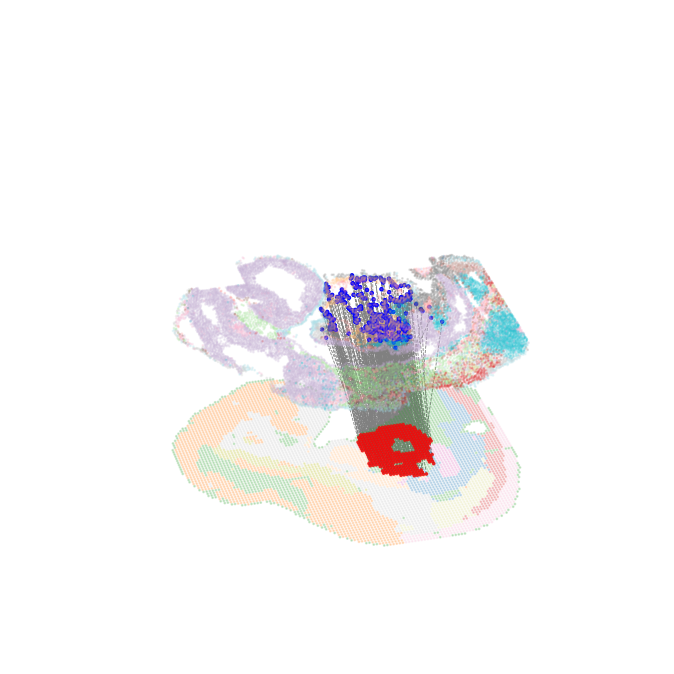
Visualize and quantify the evaluation of Neural crest region alignment results

• We follow SLAT study sets the alignment target of Neural Creas as a collection of Cranial mesoderm, Neural Crest, Surface ectorm.

all_arrow_ends,layer_1_pcloud_3D=plot_selected_cell_type_flow(pclouds_list, model, device,selected_cell_type='Neural crest',finaltruth=['Cranial mesoderm', 'Neural crest', 'Surface ectoderm'],xlim=(-0.1, 1.1),ylim=(-0.1, 1.1),height_scale=1,size=1,alpha=0.25,
    #save_path='/home/dbj/DPLFC/'
)

Number of arrow ends: 1008
Layer 1 points count: 2169

chamfer_dist = chamfer_distance(all_arrow_ends,layer_1_pcloud_3D)

print(f"chamfer distance: {chamfer_dist}")

chamfer distance: 0.005473908230508169